KAYABOARD — Magnetic-Levitation Organ Keyboard (Proof of Concept)
Research notes on keybed geometry, piano action, magnetic return force, and optical sensing
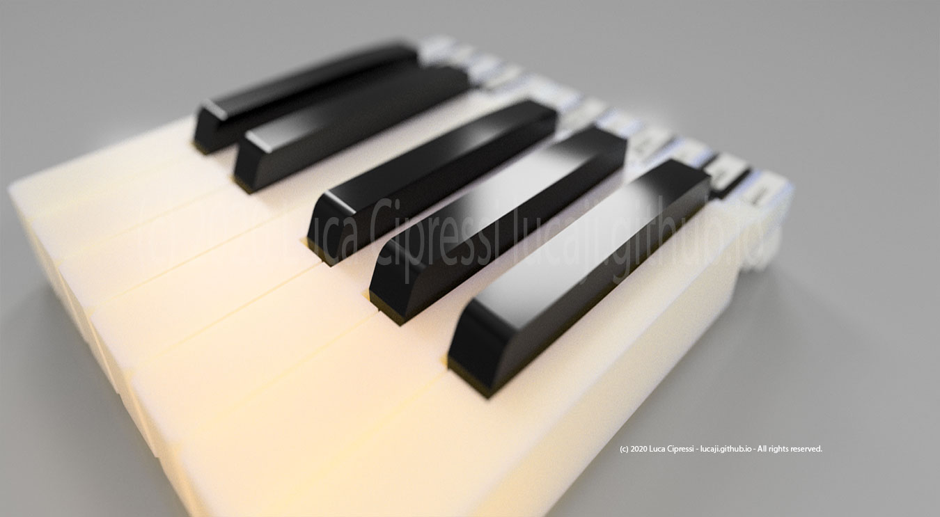
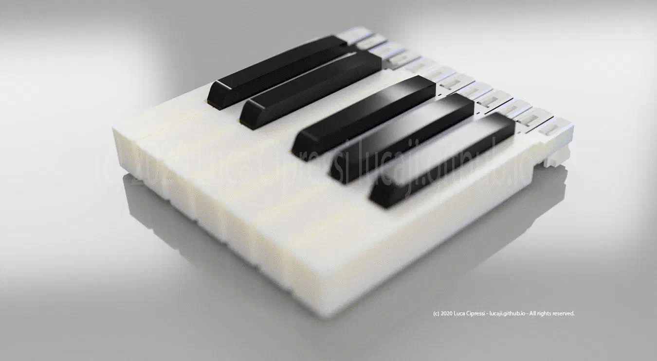
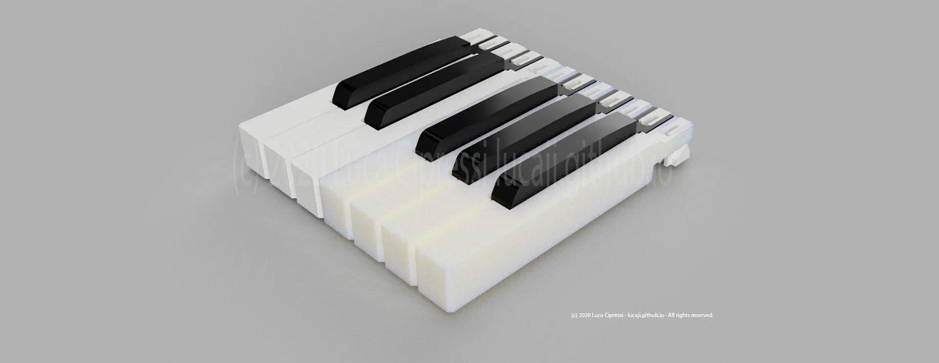
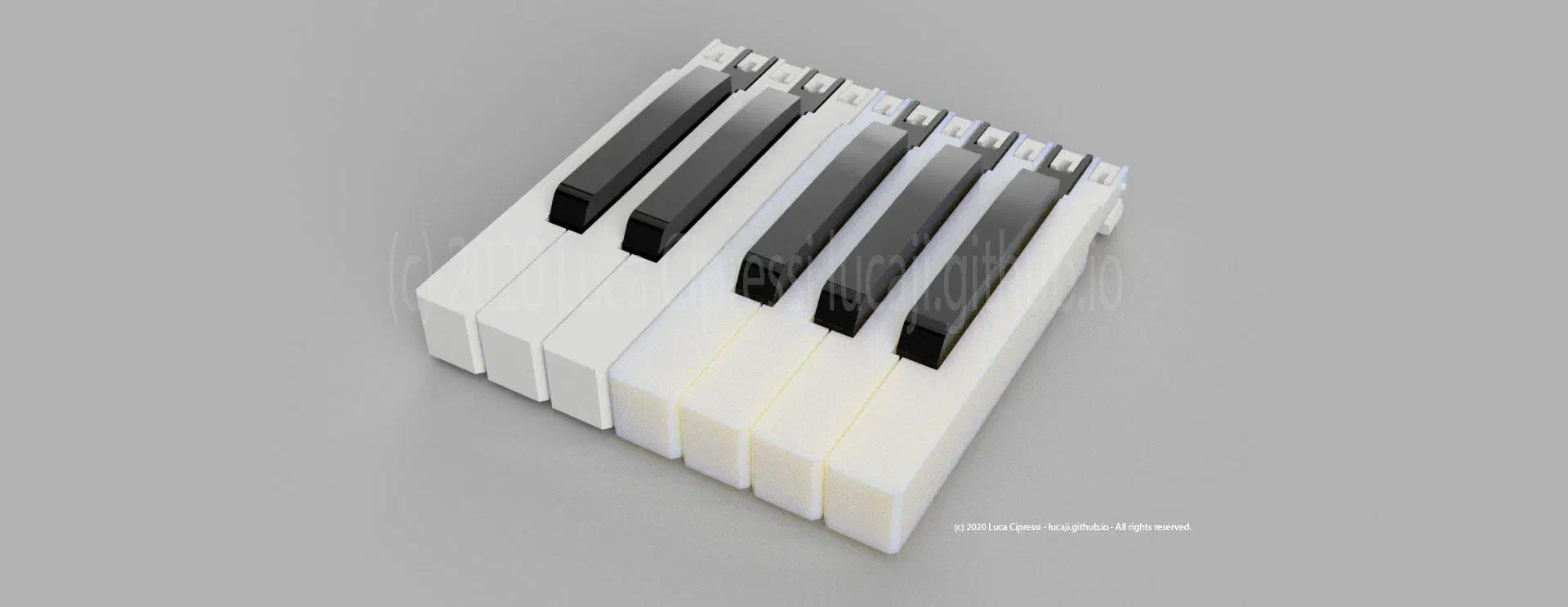
This is a proof of concept for an organ keyboard using magnets instead of conventional metal springs. The goal is not to build a free-floating magic trick, but a playable musical keybed where the return force, counter-pressure, and release behaviour can be tuned by geometry and by the distance between permanent magnets.
I started this project because I wanted a custom manual for organ and tonewheel-style instruments: a keyboard that could be fast, light, repeatable, mechanically simple, and open to experimentation. The result is KAYABOARD, a 3D model and mechanical study for a magnetic-return organ manual with optical sensing and MIDI output.
The first encouraging result is that the magnetic version can actually feel usable. After several iterations I succeeded in obtaining a decent key action: not a vague floating sensation, not a loose toy mechanism, but a controllable resistance curve that gives the finger a clear starting pressure, a short travel, a clean bottom stop, and a reliable return. The difficult part was discovering that magnets cannot simply be selected by catalogue pull-force. What matters is the entire force curve across the key travel, the lever ratio of the key, the rest gap, the bottom gap, and the way the player perceives the transition between preload, motion, trigger point, and bottoming.
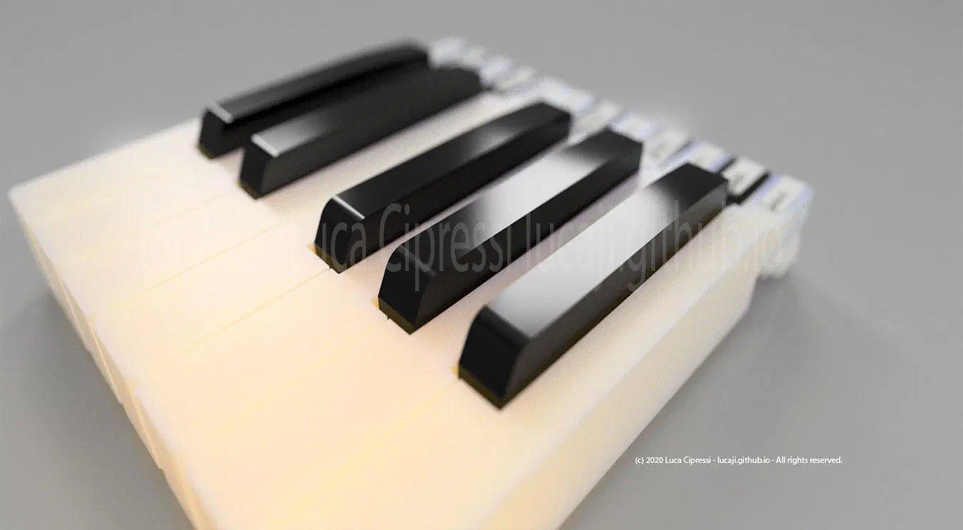
Research status
This page is a work-in-progress research paper rather than a finished build log. At this stage the project combines:
- a mechanical 3D study of the key, pivot, guide rails, stops, and magnet seats;
- research into standard piano and organ keyboard geometry;
- experiments with neodymium disc magnets as a springless return system;
- optical key sensing using IR emitter / photodiode or phototransistor pairs;
- a possible STM32-based controller for scanning, calibration, and MIDI output.
The current design target is an organ-style manual, not a weighted digital piano action. Nevertheless, the acoustic piano remains the most fascinating reference point, because its action has been refined over centuries into an extremely sensitive human interface.
Why start from the piano?
I have always admired the acoustic piano keyboard mechanics. It is a small masterpiece of leverage, inertia, escapement, friction management, felt compression, repetition, and regulation. A grand piano action is not just a switch and not simply a lever: it is a kinetic chain that lets the player accelerate a hammer toward a string and then releases it at the last moment so the string can vibrate freely.
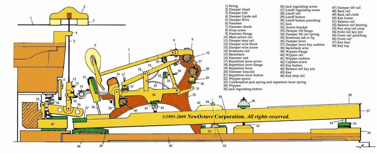
An organ manual is fundamentally different. On an organ, pressing a key opens an electrical or pneumatic path and the note continues to sound for as long as the key is held. There is no hammer, no string, no velocity-dependent acoustic excitation in the traditional pipe-organ or Hammond sense. This is why organ actions can be lighter and faster than piano actions, and why the playing technique is different.
Still, the piano offers useful lessons:
- the player’s finger expects a very repeatable travel distance;
- small variations in key dip, friction, and return force are immediately felt;
- the force should not change randomly from note to note;
- a keybed is a calibrated mechanical instrument, not merely a row of switches.
Standard keyboard geometry
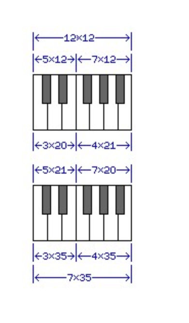
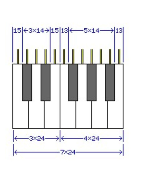
A modern full-size piano keyboard usually has 88 keys, from A0 to C8: 52 white keys and 36 black keys. Modern piano octave spans are commonly around 164–165 mm, giving a white-key pitch of roughly 23.4–23.6 mm at the front and a semitone mechanism spacing around 13.7 mm when divided across twelve notes. These values are not magic constants; they are the result of historical convergence and manufacturing practice, with small variations between makers.
The organ world uses a different range convention. A typical full organ manual is 61 notes, usually from C to C across five octaves. Many historical or smaller instruments use 56 or 58 notes. Classic Hammond consoles such as the B-3, C-3, and A-100 are associated with waterfall keys, whose flat front and rounded edge are friendly to palm smears and glissandi.
| Parameter | Typical piano reference | Typical organ / Hammond-style reference | Design implication for KAYABOARD |
|---|---|---|---|
| Compass | 88 notes, A0–C8 | often 61 notes, C–C | A 61-note manual is a practical first target. |
| Octave span | about 164–165 mm | similar musical spacing | Keep full-size spacing for transferable technique. |
| White-key pitch | about 23.5 mm | usually comparable | Front geometry should feel familiar. |
| Key travel / dip | about 9.3–10.6 mm on many grands | often around 8–12 mm depending tradition | Target around 10 mm, with adjustable stops. |
| Touch force | piano middle notes often around 45–55 g downweight | organ manuals can be lighter or intentionally firmer | Magnetic preload should be adjustable. |
| Note response | hammer velocity matters | key closure / speech point matters | Optical trigger point and release hysteresis are critical. |
A subtle but important geometrical issue is that seven white keys and twelve semitones must coexist within the same octave width. The white keys need to appear evenly spaced to the player, but the internal mechanism wants a near-even chromatic division. This is why black keys are not simply decorative objects centred visually between equal rectangles. They occupy the compromise between the player’s hand and the instrument’s internal spacing.
For KAYABOARD, I prefer to keep the front of the keyboard familiar and do most of the experimental work behind the visible playing surface: pivot position, magnet position, guide slots, optical sensing and adjustment screws can change without forcing the player’s hand to adapt to a strange layout.
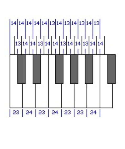
Piano action specifications as useful benchmarks
Piano regulation is the craft of adjusting the mechanical system that transfers finger motion to hammer motion. The Piano Technicians Guild describes regulation as the adjustment of the mechanical parts that cause the strings to sound and that affect the piano’s touch, responsiveness, dynamic range, and repetition.
For reference, typical grand-piano regulation values often fall into these approximate ranges:
| Regulation parameter | Typical reference value | Meaning |
|---|---|---|
| Key dip | about 9.3–10.6 mm | Total downward travel of the front of the key. |
| Hammer blow distance | about 42–48 mm | Distance from hammer rest to string before striking. |
| Let-off | about 1–3 mm | Point where the jack releases the hammer near the string. |
| Drop | often close to let-off plus a small margin | Hammer fall after escapement. |
| Aftertouch | about 0.8–1.5 mm | Remaining key travel after escapement. |
| Backcheck distance | about 13–16 mm | Hammer catch distance after the blow. |
| Downweight | often about 46–52 g, depending register and maker | Minimum weight at the key front needed to depress the key slowly. |
| Upweight | often 20 g or more | Weight the key can lift while returning. |
These figures are not universal laws. Piano actions differ by maker, size, hammer weight, leverage ratio, friction, and intended touch. Still, they offer a valuable vocabulary for this project: dip, downweight, upweight, balance weight, friction, return speed, hysteresis, and uniformity across the manual.
Downweight, upweight, balance weight, friction
A simple way to describe a key action is to measure how much weight at the front of the key makes it move down, and how much weight it can lift when returning.
Let:
- \( DW \) = downweight, in grams;
- \( UW \) = upweight, in grams.
Then two useful derived quantities are:
\[ BW = \frac{DW + UW}{2} \]
\[ F_r = \frac{DW - UW}{2} \]
where \( BW \) is the approximate balance weight and \( F_r \) is a practical estimate of friction or hysteresis in gram-force units.
For a real piano, these numbers include the weight of the key, the hammer, the wippen, felt friction, bushing friction, repetition spring influence, and geometry. For KAYABOARD, the same equations remain useful even though the mechanism is simpler: they give a language for comparing one prototype key to another.
A magnetic key can have low mechanical friction but still feel uneven if the magnet curve is too steep near the bottom of travel. Conversely, a slightly damped return can feel more expensive and controllable than a perfectly frictionless snap-back. This is one reason why the target should not be “minimum friction at all costs”; the target should be musical controllability.
Why magnets?
Traditional organ and synthesizer keybeds normally use springs, rubber domes, leaf contacts, silicone bubbles, or small mechanical return elements. Springs are simple and predictable, but their behaviour is essentially linear over the useful travel:
\[ F_s(y) = F_0 + k y \]
where \( F_s \) is the spring force, \( F_0 \) is preload, \( k \) is spring stiffness, and \( y \) is key displacement.
Magnets behave differently. Two opposing magnets can produce a smooth, contactless repulsive force. The return element does not rub, does not fatigue in the same way as a small steel spring, and can be tuned by changing:
- magnet grade, diameter, and thickness;
- axial or diametric magnetisation;
- rest gap;
- bottom gap;
- lever arm;
- magnet angle;
- use of steel backing plates;
- number of magnets per key;
- shims and adjustment screws.
This also means that magnets are unforgiving. A difference of 0.5 mm in the gap can be very obvious to the finger, especially when the magnets are small and close. The instrument is not tuned only note-by-note; it is tuned in millimetres.
Permanent magnets are not magic levitation
The term “mag-lev” is attractive, but in this project it should be understood mechanically. A key constrained by a pivot, guide rails, and stops can use magnets as a contactless return force. It is not freely levitating in space.
This distinction matters because unconstrained static levitation with permanent magnets is unstable in the general case. KAYABOARD avoids that problem by constraining the key mechanically. The magnets supply force; the keybed supplies geometry.
In other words:
- the key pivots around a known axis;
- lateral movement is controlled by guide rails or bushings;
- top and bottom travel are limited by stops;
- magnets provide a shaped vertical force curve.
The design question therefore becomes: what magnetic force curve produces a good musical key?
Magnetic force: useful formulas
The exact force between two real cylindrical neodymium magnets depends on magnet geometry, magnetisation, distance, alignment, nearby steel, and manufacturing tolerances. For design purposes, however, a few models are useful.
1. Ideal dipole approximation
At distances large compared with the magnet size, two axially aligned magnetic dipoles can be approximated as dipoles. The axial force magnitude scales approximately as the inverse fourth power of distance:
\[ F_m(g) \approx \frac{3 \mu_0 m_1 m_2}{2 \pi g^4} \]
where:
- \( F_m \) is the magnetic force in newtons;
- \( \mu_0 = 4\pi \times 10^{-7}\ \mathrm{N/A^2} \) is the permeability of free space;
- \( m_1 \) and \( m_2 \) are the magnetic dipole moments;
- \( g \) is the gap between the magnetic centres or an effective separation.
This model explains the most important practical fact: magnetic force changes very quickly with distance. If the gap is halved, the ideal dipole force rises by about \( 2^4 = 16 \). Real disc magnets at short range deviate from the ideal dipole model, but the design lesson remains valid.
2. Empirical force fit
For small keyboard magnets, the most useful engineering model is often empirical:
\[ F_m(g) = \frac{A}{(g + g_e)^n} + C \]
where:
- \( A \) is a fitted force constant;
- \( g \) is the measured face-to-face air gap;
- \( g_e \) is an effective offset that absorbs magnet thickness and non-ideal geometry;
- \( n \) is an exponent often somewhere between 2 and 4 in a limited working range;
- \( C \) is a small offset for measurement bias.
The exact exponent is less important than getting a reliable fit in the actual travel range of the key. For example, if the key moves from a 7 mm magnet gap at rest to a 3 mm gap at the bottom, only that interval matters.
3. Magnetic stiffness
The player does not feel force alone. The player feels how force changes with travel. This is stiffness:
\[ k_m(g) = -\frac{dF_m}{dg} \]
For the empirical model:
\[ k_m(g) = \frac{nA}{(g + g_e)^{n+1}} \]
The negative sign disappears in practice because the force increases as the gap decreases.
This is why a magnetic key can feel pleasant near the top but too hard near the bottom: the stiffness rises rapidly when the magnets get close. A mechanical stop with felt or elastomer becomes important because the final millimetre can otherwise feel abrupt.
4. Lever conversion from magnet force to finger force
A key is a lever. Let:
- \( L_f \) = distance from pivot to the front playing point;
- \( L_m \) = distance from pivot to the magnet force point;
- \( F_p \) = force applied by the player at the key front;
- \( F_m \) = magnetic force at the magnet;
- \( \theta \) = key rotation angle.
Static torque balance gives:
\[ F_p L_f \approx F_m L_m + \tau_w + \tau_f \]
where \( \tau_w \) includes key weight and counterweight torque, and \( \tau_f \) includes friction or hysteresis.
Ignoring weight and friction for a first estimate:
\[ F_p \approx F_m \frac{L_m}{L_f} \]
If the magnet is halfway between pivot and key front, only about half the magnet force is felt at the finger. If the magnet is close to the pivot, a strong magnet may still feel light. If the magnet is too close to the front, a small gap error becomes very noticeable.
5. Gap as a function of key travel
For small rotations:
\[ \theta \approx \frac{y_f}{L_f} \]
where \( y_f \) is the vertical travel at the key front.
If the magnet is located at \( L_m \), the vertical displacement at the magnet is approximately:
\[ y_m \approx L_m \theta = y_f \frac{L_m}{L_f} \]
For a repelling pair whose gap decreases as the key is pressed:
\[ g(y_f) = g_0 - y_f \frac{L_m}{L_f} \]
where \( g_0 \) is the rest gap.
Combining this with the empirical magnetic model gives a key-front force curve:
\[ F_p(y_f) \approx \frac{L_m}{L_f} \cdot \frac{A}{\left(g_0 - y_f \frac{L_m}{L_f} + g_e\right)^n} \]
This formula is extremely useful because it shows the available tuning parameters:
- increase \( g_0 \) to lighten the key;
- decrease \( g_0 \) to increase preload;
- reduce \( L_m/L_f \) to soften the felt force curve;
- choose a smaller magnet or lower grade to reduce \( A \);
- prevent \( g(y_f) \) from becoming too small near the bottom.
6. Effective key stiffness at the finger
Differentiating the key-front force with respect to key-front displacement gives:
\[ k_p(y_f) = \left(\frac{L_m}{L_f}\right)^2 \frac{nA}{\left(g_0 - y_f \frac{L_m}{L_f} + g_e\right)^{n+1}} \]
This square term is important. Moving the magnet closer to the pivot reduces both force and stiffness at the finger. That makes magnet placement one of the most powerful design controls.
A practical calibration method
The best results so far came from treating the magnetic action as something to regulate, just like a small piano action, rather than something to merely assemble.
Step 1 — define the target travel
For the current prototype I would start with:
| Parameter | Starting target |
|---|---|
| Front key dip | 9.5–10.5 mm |
| Trigger point | 40–60% of travel |
| Bottom felt compression | 0.5–1.0 mm |
| Release point | slightly above trigger point to create hysteresis |
| Return time | fast enough for repeated notes without bouncing |
| Note-to-note force variation | ideally within a few gram-force after calibration |
For an organ controller, velocity can be optional. A Hammond-style tonewheel emulation does not need strike velocity to define loudness, but velocity data may still be useful for external MIDI instruments or for experimental percussion/organ hybrid patches.
Step 2 — measure the magnet pair outside the keyboard
A very simple jig can be enough:
- fix one magnet to a rigid base;
- mount the opposing magnet on a vertical slider;
- place the assembly on a digital scale or load cell;
- insert calibrated spacers: 2 mm, 3 mm, 4 mm, 5 mm, etc.;
- record force at each gap;
- repeat the measurement while approaching and leaving the gap to detect mechanical friction in the jig.
Convert grams to newtons with:
\[ F[\mathrm{N}] = m[\mathrm{g}] \cdot \frac{9.80665}{1000} \]
Then fit the data to:
\[ F_m(g) = \frac{A}{(g + g_e)^n} + C \]
The fitted curve is more useful than the magnet catalogue number. Pull-force values are usually measured against thick steel in ideal conditions, while this keyboard uses magnet-to-magnet repulsion or attraction at specific short gaps.
Step 3 — convert magnet force to key-front force
Use the lever ratio:
\[ F_p(g) \approx F_m(g) \frac{L_m}{L_f} \]
Then convert back to gram-force for intuitive comparison:
\[ m_p[\mathrm{g}] = \frac{1000 F_p[\mathrm{N}]}{9.80665} \]
This gives a predicted downweight curve. The curve should then be checked with real weights at the key front.
Step 4 — regulate the rest gap
The rest gap is the most sensitive adjustment. Possible methods:
- printed shims under the fixed magnet;
- threaded magnet carrier;
- small screw pressing on a magnet cradle;
- exchangeable magnet seats with different depths;
- top stop and bottom stop adjustment.
The top stop defines the rest position and therefore the preload. The bottom stop defines the minimum magnet gap. Both must be stable. A bottom stop that lets the magnets get too close creates a harsh rise in force and can also make the key noisy.
Step 5 — measure downweight and upweight
For each key:
- place gram weights at the usual front playing point;
- add weight until the key slowly begins to descend: this is \( DW \);
- from the depressed state, remove weight until the key begins to rise: this is \( UW \);
- compute \( BW \) and \( F_r \);
- adjust the magnet gap or add damping if the values are inconsistent.
A prototype calibration table could look like this:
| Note | Rest gap | Bottom gap | Dip | DW | UW | BW | Friction / hysteresis | Trigger travel | Return quality |
|---|---|---|---|---|---|---|---|---|---|
| C2 | 6.0 mm | 3.5 mm | 10.0 mm | 72 g | 34 g | 53 g | 19 g | 5.0 mm | clean |
| C3 | 6.1 mm | 3.6 mm | 10.0 mm | 70 g | 35 g | 52.5 g | 17.5 g | 5.0 mm | clean |
| C4 | 6.0 mm | 3.5 mm | 10.0 mm | 71 g | 36 g | 53.5 g | 17.5 g | 5.0 mm | slight bounce |
These numbers are illustrative placeholders, not final KAYABOARD specifications. The important point is to measure and regulate the curve key by key.
Step 6 — calibrate the sensor
With an optical sensor, the key has both a mechanical curve and an electrical curve. The firmware should store at least:
- raw sensor value at rest;
- raw sensor value at bottom;
- trigger threshold;
- release threshold;
- optional velocity thresholds;
- dead zone near rest;
- debounce or hysteresis value.
For a continuous optical reading:
\[ x = \frac{ADC - ADC_{rest}}{ADC_{bottom} - ADC_{rest}} \]
where \( x \) is normalized key travel from 0 to 1.
A simple trigger rule is:
\[ note_on \quad \text{if} \quad x > x_{on} \]
\[ note_off \quad \text{if} \quad x < x_{off} \]
with:
\[ x_{off} < x_{on} \]
The separation between \( x_{on} \) and \( x_{off} \) prevents chatter around the switching point.
For MIDI velocity experiments:
\[ v = \frac{x_2 - x_1}{t_2 - t_1} \]
\[ V_{MIDI} = 1 + 126 \cdot \left( \frac{v - v_{min}}{v_{max} - v_{min}} \right)^\gamma \]
where \( \gamma \) controls the response curve. For organ playing, \( V_{MIDI} \) can simply be fixed at 100 or 127, while the same keybed can still transmit velocity when used as a general MIDI controller.
What made the magnetic action feel decent
The working lesson was that the action improved when I stopped thinking of the magnets as binary “repel strongly / repel weakly” devices and started thinking in terms of force shaping.
The pleasant range came from balancing these elements:
- enough preload at rest so the key does not feel loose;
- not too much preload, otherwise the first touch feels stubborn;
- a moderate force increase through the middle of travel;
- a bottom stop that prevents the steepest part of the magnetic curve;
- a small amount of mechanical damping or felt compliance;
- repeatable magnet placement from key to key;
- enough clearance to avoid sideways magnetic pull and rubbing.
In practice, a magnetic keybed is more like regulating a set of tiny magnetic springs than levitating a piano. Every key has a return curve, and the player’s hand immediately notices the outliers.
Optical sensing
The current concept uses an IR emitter and photodiode/phototransistor pair across each key slot. The moving key interrupts or reflects the light, producing a raw analog or digital value.
Possible sensing strategies:
| Sensor strategy | Advantage | Disadvantage |
|---|---|---|
| Simple digital interruption | easy scanning, low cost | only on/off, no velocity unless two points are used |
| Analog optical travel | continuous position, velocity possible | needs calibration and shielding from ambient light |
| Hall sensor with magnet | robust and contactless | magnetic return system may interfere unless separated |
| Conductive rubber / contact | proven and cheap | contact wear and less experimental value |
| Capacitive sensing | no optical alignment | more sensitive to grounding and environment |
Because the key already contains magnets, Hall sensing is tempting, but it complicates the magnetic-field layout. Optical sensing keeps the force system and the sensing system more independent.
Controller notes
The controller can be based on an STM32 microcontroller scanning either digital inputs or multiplexed analog channels. The intended outputs are:
- USB MIDI;
- optional USB CDC debug interface;
- optional traditional 5-pin DIN MIDI;
- calibration storage in flash or external EEPROM;
- per-key curves and thresholds.
A minimal firmware architecture:
- scan all raw key sensors;
- normalize each key using stored rest/bottom calibration;
- apply hysteresis;
- compute note-on and note-off events;
- compute optional velocity;
- send MIDI;
- expose a calibration mode over serial or USB.
Pseudo-logic for one key:
x = normalize(adc_value, key.rest, key.bottom);

if (!key.down && x > key.on_threshold) {
    velocity = compute_velocity(key.history);
    midi_note_on(key.note, velocity);
    key.down = true;
}

if (key.down && x < key.off_threshold) {
    midi_note_off(key.note);
    key.down = false;
}
The most important firmware feature is not complexity but repeatability. A beautifully printed keybed will still feel bad if the switching points vary randomly from key to key.
Design notes for the next prototype
The next KAYABOARD iteration should include:
- adjustable top stop for each key;
- adjustable or shimmed bottom stop;
- fixed datum surface for measuring key height;
- replaceable magnet carriers;
- enough room to change magnet diameter or thickness;
- printed test key with exposed magnet mount for force measurement;
- a calibration jig that measures key force and sensor value simultaneously;
- mechanical damping at the bottom of travel;
- shielding or baffling for optical sensors;
- a service mode that prints raw sensor values and detected travel.
A useful future experiment would be to print only one octave and regulate it carefully before committing to a complete 61-note manual. One octave is enough to test hand feel, glissando behaviour, black-key clearance, return speed, and calibration repeatability.
Safety notes
Neodymium magnets can pinch skin, shatter if they snap together, damage magnetic storage media, and interfere with some medical devices. Small magnets are also dangerous if swallowed. During prototyping, magnets should be handled with spacers, eye protection, and a clean bench free of loose steel tools.
The musical instrument may be playful; the magnets are not toys.
Conclusion
KAYABOARD began as a 3D study of a springless organ manual and has become a small research project about musical touch. The acoustic piano remains the benchmark for mechanical refinement, while the organ provides the target behaviour: fast, repeatable, expressive keying without the mass and escapement of a hammer action.
The magnetic version is promising because it gives a clean, adjustable, contactless return force. The challenge is that magnetic force is highly nonlinear. This means the project cannot be solved by choosing “strong enough” magnets. It must be solved by measuring, fitting, regulating, and calibrating the complete key system.
That is the next phase: one key, then one octave, then a complete manual.
References and further reading
- The Size of the Piano Keyboard — Quadibloc
- Piano Keyboards — DataGenetics
- Action Regulation — Piano Technicians Guild
- Grand Piano Regulation Specifications — 88Keys
- Kawai Grand Piano Regulation Manual
- Action Regulation Specifications — The Definitive Steinway Reference
- A Guide to Piano Key Measurements and Renner’s KMD — World Piano News
- The Stanwood New Action Protocol for Grand Pianos — Piano Congress
- Grand Regulation: Key Dip — Grandwork Tools
- Waterfall Keys — HammondWiki
- Keyboards and Consoles — Organ Historical Society
- British Organ Console Dimensions — OrganWorks
- Magnet Pull Force Calculator — K&J Magnetics
- Magnet Gap Calculator — K&J Magnetics
- Guide to Measuring Magnetic Strength — K&J Magnetics
- Closed-form equations for force between cylindrical magnets — Encyclopedia Magnetica